Analyzing Murdock (1962) Free Recall Data
This tutorial demonstrates analyzing the classic Murdock (1962) free recall dataset, which established the serial position effect as a fundamental phenomenon in memory research.
The dataset contains 90 subjects (15 per condition) across 6 experimental conditions varying in list length (10, 15, 20, 30, or 40 items) and presentation rate (1 or 2 sec/item). Each subject completed 80 lists.
Conditions:
LL10-2s: 10 items, 2 sec/item (15 subjects, 80 lists each)
LL15-2s: 15 items, 2 sec/item (15 subjects, 80 lists each)
LL20-1s: 20 items, 1 sec/item (15 subjects, 80 lists each)
LL20-2s: 20 items, 2 sec/item (15 subjects, 80 lists each)
LL30-1s: 30 items, 1 sec/item (15 subjects, 80 lists each)
LL40-1s: 40 items, 1 sec/item (15 subjects, 80 lists each)
We’ll analyze recall performance using:
Probability of First Recall (PFR) - probability of recalling each position first
Lag-CRP - conditional recall probability by temporal lag
Serial Position Curve (SPC) - recall probability by encoding position
Reference: Murdock, B. B. (1962). The serial position effect of free recall. Journal of Experimental Psychology, 64(5), 482-488. https://doi.org/10.1037/h0045106
[1]:
import quail
import matplotlib.pyplot as plt
import warnings

# Suppress RuntimeWarnings about empty slices
warnings.filterwarnings('ignore', category=RuntimeWarning)
Load the dataset
The Murdock 1962 dataset is included with quail and can be loaded using load_example_data().
[2]:
# Load the Murdock 1962 dataset
egg = quail.load_example_data('murd62')

print(f"Loaded Murdock 1962 data: {egg.n_subjects} subjects, {egg.n_lists} lists per subject")
Loaded Murdock 1962 data: 90 subjects, 80 lists per subject
Set up subject groupings
Since each subject belongs to a single condition, we create a subjgroup list that maps each subject to their condition. This allows us to plot separate curves for each condition.
[3]:
# Build subjgroup: map each subject index to its condition name
subjgroup = []
for subj_idx in range(egg.n_subjects):
    try:
        sample = egg.pres.loc[(subj_idx, 0)][0]
        if sample and 'condition' in sample:
            subjgroup.append(sample['condition'])
        else:
            subjgroup.append('Unknown')
    except (KeyError, IndexError, TypeError):
        subjgroup.append('Unknown')

print(f"Subject conditions: {len(set(subjgroup))} unique conditions")

# Create listgroup for averaging across lists within each subject
listgroup = ['average'] * egg.n_lists
Subject conditions: 1 unique conditions
Analyze and plot
We’ll create three plots showing key memory phenomena:
PFR: Shows the primacy effect - items at the beginning of a list are more likely to be recalled first
Lag-CRP: Shows temporal contiguity - items studied close together are likely to be recalled together
SPC: Shows the classic serial position curve with primacy and recency effects
[4]:
# Create figure with 3 subplots in order: PFR, Lag-CRP, SPC
fig, axes = plt.subplots(1, 3, figsize=(15, 5))

# 1. Probability of First Recall - use quail's built-in plot with error bars
pfr = egg.analyze('pfr', listgroup=listgroup)
pfr.plot(ax=axes[0], subjgroup=subjgroup, plot_type='subject', legend=True)

# 2. Lag-CRP - use quail's built-in plot with error bars (legend=False)
lagcrp = egg.analyze('lagcrp', listgroup=listgroup)
lagcrp.plot(ax=axes[1], subjgroup=subjgroup, plot_type='subject', legend=False)

# 3. Serial Position Curve - use quail's built-in plot with error bars (legend=False)
spc = egg.analyze('spc', listgroup=listgroup)
spc.plot(ax=axes[2], subjgroup=subjgroup, plot_type='subject', legend=False)

# Configure PFR plot
axes[0].set_title('Probability of First Recall')
axes[0].set_xlabel('Serial Position')
axes[0].set_ylabel('Probability')
axes[0].set_ylim([0, 0.6])

# Configure Lag-CRP plot
axes[1].set_title('Lag-CRP')
axes[1].set_xlabel('Lag')
axes[1].set_ylabel('Conditional Recall Probability')
axes[1].set_xlim([-10, 10])
axes[1].set_ylim([0, 0.5])
axes[1].axvline(x=0, color='gray', linestyle='--', alpha=0.5)

# Configure SPC plot
axes[2].set_title('Serial Position Curve')
axes[2].set_xlabel('Serial Position')
axes[2].set_ylabel('Recall Probability')
axes[2].set_ylim([0, 1])

plt.tight_layout()
plt.suptitle('Murdock (1962) Free Recall Data', y=1.02, fontsize=14)
plt.show()
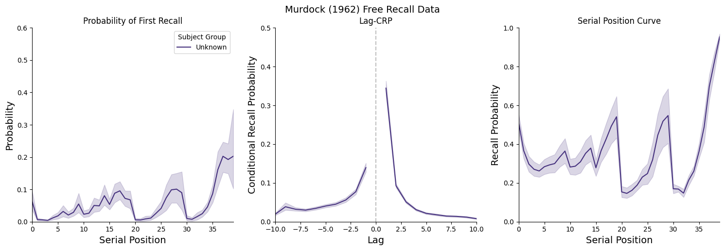
Key findings
The plots reveal several classic memory phenomena:
Primacy Effect: Items at the beginning of the list are recalled more often (visible in SPC)
Recency Effect: Items at the end of the list are recalled more often (visible in SPC)
Temporal Contiguity: Items studied nearby in time tend to be recalled together (visible in Lag-CRP asymmetry toward +1 lag)
List Length Effects: Longer lists show lower overall recall probability but similar curve shapes